
This page holds preliminary results - this data has not been validated yet (in progress!!)
Material on this page was last updated: 8/9/2017
Please refer to the following pages for further information related to :
This page provides preliminary results of a performance analysis of the SC-CVT. The contents should be viewed as preliminary data - we have not validated the results. We post this page to provide an illustration of our current direction. The raw data used for the figures can be found at https://people.cs.clemson.edu/~jmarty/research/ConnectedVehicle/results/. In particular,
Figure 1 illustrates the SC-SCT system. The deployment consists of three nodes that house a Road Side Unit (RSU). We have a number of On Board Units that we use in vehicles for test purposes.
Figure 2 provides further details of the system. The system, which consists of hardware and software, is an implementation of a software architecture designed to facilitate our research in the area of Connected Vehicles and more broadly the Internet of Things. The system supports a set of nodes including mobile edge nodes, fixed edge nodes and system nodes. In a Connected Vehicle (CV) context, the mobile edge nodes contain an OBU along with an processor board that can support additional connectivies through USB dongles. Fixed edge nodes contain a RSU. A system node represents are more functional 'backend' node. The mobile and fixed edge nodes support a standards based DSRC/WAVE environment. In parallel, the system supports an experimental framework that extends a WAVE environment with an IoT framework that we have developed. This framework, referred to as ThinGs In a Fog (TGIF), provides an object oriented interface to TGIF applications to make use of system services for messaging, location, networking, and security. The system is under development and a limited subset of function is available on the testbed.
Figure 1. SC-CVT Deployment

Figure 2. System Model
Our evaluation includes three environments:

figure 3. Lab Environment
Figure 3 illustrates the Lab environment. Table 1 identifies a set of experiments that have been performed in the Lab environment, modeling a simple three node scenario (as illustrated in Figure 3a.). We describe one specific experiment- referred to as Test 14. The data is located here. We have implemented a simple UDP client server tool that can send a constant stream of UDP packets. The server side simply observes the arrivals and monitors the throughput, latency, and loss. Table 1 summarizes the results.
Table 1. Lab experiments
Test Id : Experiment |
Description |
perfClient send rate Setting actual (Mbps) |
Rx throughput |
Rx Loss Rate |
Interarrival Time: min/max/mean/median |
Other info |
Test 1 : Exp 0 |
Reference over wired network, UDP |
6.0 5.89 |
5.89 |
0 |
0.000024 0.001906 0.001359 0.001349 |
|
Test2 : Exp 1 |
2 OBU’s |
6.0 5.50 |
4.33 |
0.133 |
0.000059 0.015909 0.001683 0.001681 |
Profile 3 |
Test 2: Exp 2 |
2 OBU’s plus 1 malicious OBU |
6.0 5.64 |
1.92 |
0.595 |
0.000117 0.019806 0.003511 0.003246 |
Profile 3 |
Test 2: Exp 3 |
2 OBU’s plus 1 malicious OBU |
0.80 0.79 |
0.71 |
0.105 |
0.000879 0.046414 0.011265 0.010134 |
Profile 3 |
Experiment 0 provides a reference for the results by performing the experiment method with two Linux nodes connected by a gigabit Ethernet. The client (referred to as the perfClient) is instructed to send at a fixed rate of 6 Mbps. The message size is 1000 application bytes. IPv4 addressing is specified. The actual send rate differs slightly from the configured send rate due to program overhead. The server (referred to as perfServ) observes the expected arrival rate of 5.89 Mbps. The observed loss rate is 0. The Internal arrival time distribution is summarized. A median of 0.001349 seconds is very close to the mean of 0.001259 seconds suggesting there is only a small amount of jitter.
We repeat this experiment three times over the network shown in figure 3. In all cases, we have configured the OBUs for IPV4 operation over channel 180 using their second radio. We have disabled the WAVE stack on the OBUs. The OBUs are configured to operate using a code rate and modulation of 1/2 QPSK. The theoretic maximum supported data rate is 6 Mbps.
The perfClient runs on obu2 and specifies the DSRC network IPv4 broadcast address of 192.168.234.255 and is instructed to use port 5000. The perfServ is coded to receive a UDB broadcast packets destined for port 5000. The perfClient's observed sending rate of 5.5 Mbps is less than what is expected. The perfServer receives packets at a rate of 4.33 Mbps with an average loss rate of 0.133. Experiment 2 repeats the method but involves a third OBU that is also running the perfClient application in a manner that is identical to OBU2 but it uses a bogus UDP port (port number 5002). In summary, this is a simple experiment involving two competing flows that both are trying to send at the highest possible rate. Flow 2 (sourced by OBU3) starts first, and then Flow 1 (sourced by OBU2) starts. We observe a significant reduction in throughput in Flow 1, with a loss rate of .595. Finally, Experiment 3 repeats Experiment 2 except Flow 1 is configured to emulate a BSM broadcast by sending a message every 100 ms. The perfClient is configured to send at a rate of 800 Kbps which leads to a 1000 byte message to be sent every 100 ms. The perfServer observes a stream arrival rate of 710Kbps with an average packet loss rate of 0.105. We did confirm that if just the BSM stream is active, without the addition stream from OBU3, the perfServer running at OBU1 receives the stream at a rate of 800Kbps with 0% packet loss.
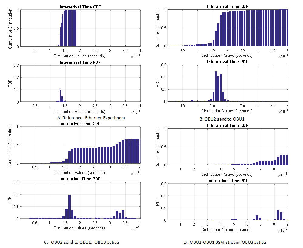
Figure 4. Arrival distribution of the four experiments
We summarize the results as follows. A 1000 byte message size using IPv4 corresponds to an Ethernet frame of size of 1056 bytes. At 6 Mbps, this corresponds to a frame sent roughly every 1.33 ms.The application does not take into account frame overhead, and so it should result in a send rate slightly larger than 6 Mbps. We are investigating the following:
There are clearly pieces of information that are needed to be able to better comprehend these results. In a future update to this page, we will provide further information such as the results observed by Flow 2 and internal statistics made available from the OBUs including the channel utilization, frame counts, collision rates. Further, Experiment 3, we will reduce the BSM message size to a value that is comparable to a WAVE. We will also reproduce the experiment when OBUs 1 and 2 are configured in WAVE mode to send correct BSM messages (38 bytes) every 100 ms.
One of the results we are targeting is to be able to characterize normal operation in a DSRC network so that it might be possible to identify (classify) malicious or erroneous behaviors. This represents our ongoing work.